Reading the Snowflake Query Profile: Where the Credits Actually Go
How I read the operator tree: TableScan bytes, partition pruning, local and remote spilling, and the exchange steps that quietly dominate runtime.
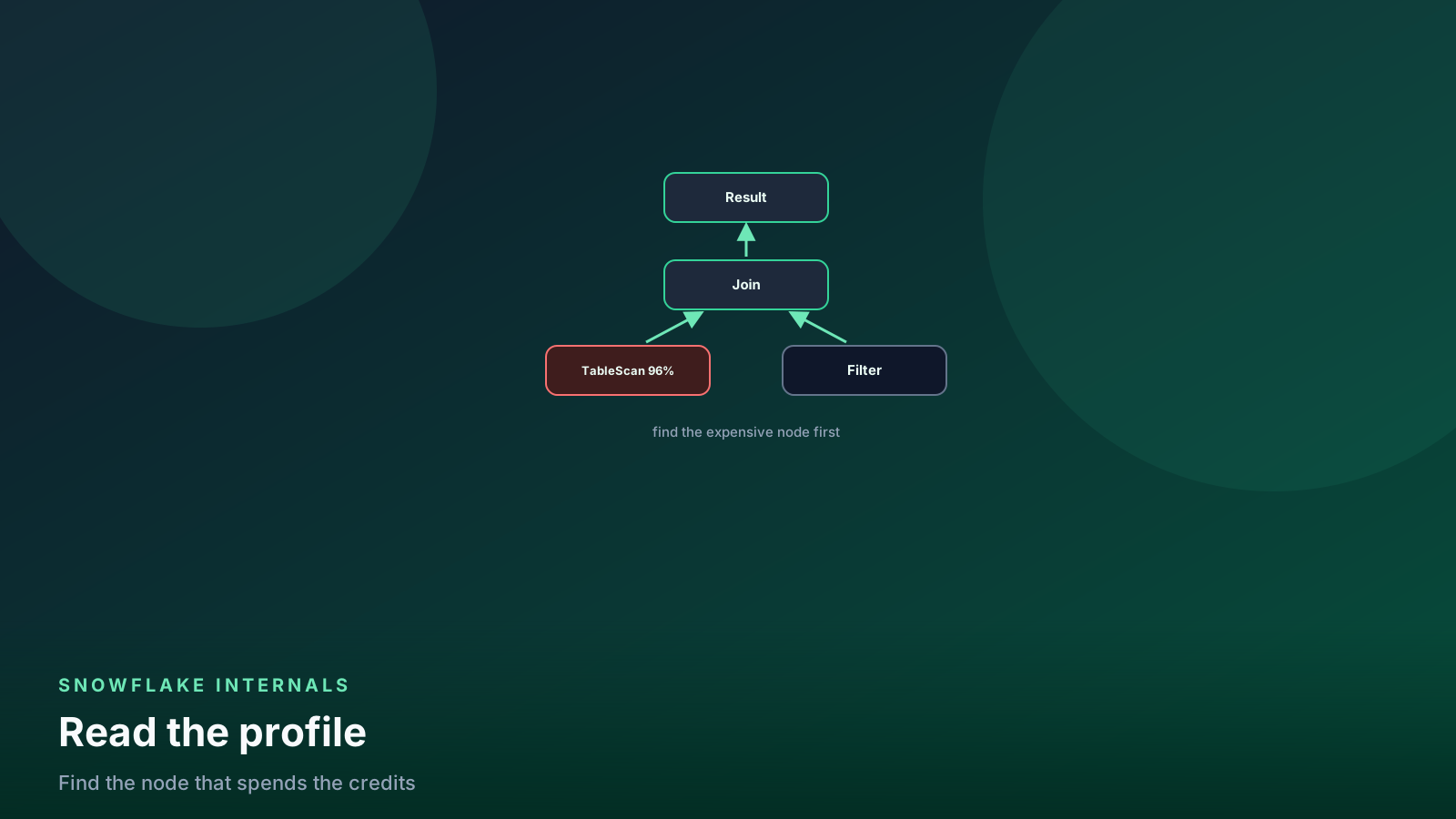
- ✓The operator tree tells you where time went. The SQL text tells you almost nothing.
- ✓Partitions scanned vs partitions total is the first number I read. Bad pruning is the most common root cause.
- ✓Remote spilling means the warehouse is too small for the join or sort. Local spilling is a warning, remote is a bill.
- ✓A fat exchange between operators usually means a join exploded or a bad distribution, not a slow scan.
- ✓GET_QUERY_OPERATOR_STATS lets you read profiles in SQL, so you can hunt regressions across a whole workload.
Table of contents
The slowest part of most Snowflake debugging sessions is the part where someone stares at the SQL. The SQL is the plan’s input, not the plan. When a query takes eleven minutes and someone asks why, the answer is in the Query Profile, and it is usually one of three things: a scan that pruned nothing, a join that exploded, or a sort that spilled to remote storage.
I read profiles the same way every time. Find the most expensive operator. Check whether the scan pruned. Check whether anything spilled. Check the row counts flowing between operators. That order resolves the majority of incidents before anyone suggests resizing the warehouse — which is the expensive way of not reading the profile. If cost is the symptom, start with the cost optimization guide; if a specific query is the symptom, start here.
flowchart TD
  q[Slow query] --> op["Most expensive operator?"]
  op --> scan["TableScan: check partitions scanned"]
  op --> join["Join: check output vs input rows"]
  op --> sort["Sort or Aggregate: check spilling"]
  scan --> prune["Bad pruning: fix predicate or clustering"]
  join --> explode["Row explosion: fix join keys"]
  sort --> spill["Remote spill: reduce data or resize"]
The three roads a slow query takes. The profile tells you which one within a minute.
Getting to the profile
In Snowsight, open Query History, click the query, open the Query Profile tab. You get the operator tree, a percentage of total time per operator, and statistics panels per node. The percentages are the map. Anything above 20 percent of total time deserves a click.
For anything systematic, skip the UI. The operator stats are available as a table function, which means you can read a profile with SQL and join it to history:
select
  operator_id,
  parent_operators,
  operator_type,
  operator_statistics:input_rows::number as input_rows,
  operator_statistics:output_rows::number as output_rows,
  execution_time_breakdown:overall_percentage::float as pct_of_query,
  operator_statistics:pruning:partitions_scanned::number as partitions_scanned,
  operator_statistics:pruning:partitions_total::number as partitions_total,
  operator_statistics:spilling:bytes_spilled_local_storage::number as spill_local,
  operator_statistics:spilling:bytes_spilled_remote_storage::number as spill_remote
from table(get_query_operator_stats('01b7c2ae-0604-9d3f-0000-0d2500a1b2c3'))
order by pct_of_query desc;
This is the function I wish more teams knew about. It turns “open forty profiles by hand” into a query. When a dashboard got slow last quarter, I ran this across every query ID from the offending Looker user and grouped by operator type. The answer was a single TableScan that had stopped pruning after a schema change. Nobody would have found that clicking through Snowsight.
TableScan: the pruning check
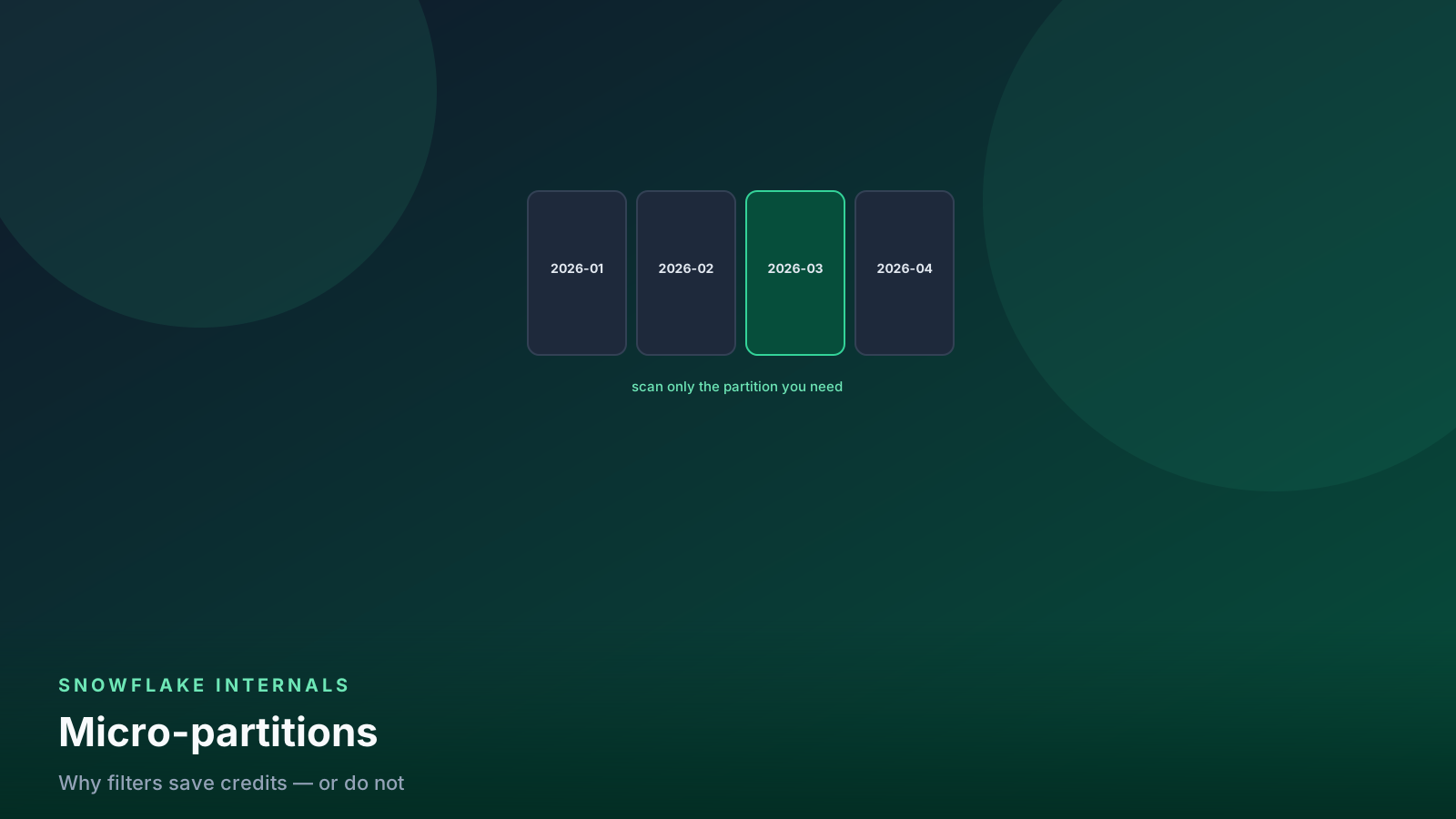
Every TableScan node reports partitions scanned and partitions total. Those two numbers are the health of your physical layout. Scanning 118 of 41,000 micro-partitions is a query that will stay fast. Scanning 39,000 of 41,000 is a full table scan wearing a WHERE clause as a costume.
Pruning fails for boring reasons. A predicate wrapped in a
function — where to_date(created_at) = '2026-04-01' — can defeat
pruning that the bare column would get. A join filter that the
optimizer cannot push down. A high-cardinality filter on a column
the table is not organized by, which is the
micro-partitions and pruning
story in full.
The bytes matter as much as the partition counts. A scan can prune well and still move 800 GB because the table is wide and you selected every column. Percentage scanned tells you about layout; bytes scanned tells you about the SELECT list. Fix them separately.
If the same table keeps failing the pruning check on the same predicate, that is when clustering keys or the Search Optimization Service enter the conversation — after the profile proves the scan is the problem, not before.
Joins: watch the row counts, not the join type
The profile shows input and output rows on every operator. A join
that takes 40 million rows on one side, 2 million on the other,
and emits 900 million rows is not slow because Snowflake is slow.
It is slow because the join keys are not what you think they are.
Duplicate keys on both sides multiply. I have watched a “one to
one” join on order_id become many-to-many because a backfill
doubled rows in silver and nobody deduplicated.
The check is mechanical. Output rows should be explainable from input rows. If they are not, run the cardinality query before touching anything else:
select
  order_id,
  count(*) as dup_count
from analytics.silver.orders
group by order_id
having count(*) > 1
order by dup_count desc
limit 20;
The other join smell is a build side that is too big. Snowflake hash joins build on one side and probe with the other. When the build side does not fit in memory, you get spilling on the join node, and the fix is usually filtering that side earlier — not a bigger warehouse.
Spilling: local is a warning, remote is a bill
When an operator’s working set exceeds warehouse memory, Snowflake spills to local SSD. When it exceeds local SSD, it spills to remote storage. Local spilling costs you some speed. Remote spilling costs you a lot of speed, because every spilled byte makes a round trip to object storage, and the operator does it repeatedly.
flowchart LR
  mem[Warehouse memory] -->|overflow| local["Local SSD spill"]
  local -->|overflow| remote["Remote storage spill"]
  remote --> slow["Runtime multiplies and credits follow"]
Each overflow tier is roughly an order of magnitude slower than the one above it.
Remote spilling is one of the two legitimate reasons to size up a warehouse (the other is genuine parallelism on huge scans). Memory scales with warehouse size, so one size up often eliminates the spill and the query gets faster by more than 2x — which can make the bigger warehouse cheaper in credits, since credits are size times duration.
But resize last. First ask why the working set is so big. A sort
for a window function over the whole table, an order by feeding
a dashboard that reads 200 rows, a join that exploded upstream —
all of these shrink the working set for free. You can find chronic
spillers across the account without opening a single profile:
select
  query_id,
  user_name,
  warehouse_name,
  warehouse_size,
  round(bytes_spilled_to_local_storage / power(1024, 3), 1) as local_gb,
  round(bytes_spilled_to_remote_storage / power(1024, 3), 1) as remote_gb,
  round(total_elapsed_time / 1000 / 60, 1) as minutes
from snowflake.account_usage.query_history
where start_time > dateadd('day', -7, current_timestamp())
  and bytes_spilled_to_remote_storage > 0
order by bytes_spilled_to_remote_storage desc
limit 50;
I run this weekly. The same five queries show up every time, and they are worth more than any warehouse policy.
Exchange and the parts nobody reads
Between operators, data moves. On multi-cluster plans that shows up as exchange steps, and a fat exchange — gigabytes flowing between a scan and a join — usually means the explosion already happened below it. The exchange is the messenger. Read the operator underneath.
Two panels people skip and should not. First, the profile’s breakdown of processing versus I/O versus synchronization per operator: an operator that is 90 percent “waiting” is starved by its children, so the problem is downstream in the tree. Second, the queued time on the query itself. A query that queued for four minutes and ran for one does not have a plan problem; it has a warehouse concurrency problem, and no amount of SQL tuning fixes queueing.
Also check whether the query ran at all. A result served from the result cache shows a trivial profile. Knowing which cache hit saves you from tuning a query that never executed.
Pitfalls
Tuning the SQL before reading the profile. Rewriting a CTE into a subquery because a blog post said CTEs are slow. The optimizer inlines most of them. Read the tree first.
Resizing on the first slow query. Size fixes remote spilling and wide scans. It does not fix bad pruning, exploded joins, or queueing. Three of those four are more common.
Reading percentages without row counts. An operator at 60 percent of runtime with sane rows in and out is just doing the work. An operator at 15 percent emitting 40x its input is the actual bug.
Ignoring queued time. The profile only covers execution. If the query sat in a queue, the profile will look innocent and the user will still be angry.
Comparing runs across cache states. The second run hit the
warehouse cache. Benchmark with ALTER SESSION SET USE_CACHED_RESULT = FALSE and a warm-versus-cold note, or your
before-and-after is fiction.
FAQ
Where do I find the profile for a query that already ran?
Query History in Snowsight, or GET_QUERY_OPERATOR_STATS with the
query ID. Both work for any query within the history retention
window, not just your own — subject to role access.
What is a good partitions-scanned ratio? There is no universal number, but I get suspicious above 30-40 percent on a selective query. On a full aggregation, scanning everything is correct. The ratio is only meaningful relative to how selective the predicate should be.
Is local spilling worth fixing? Sometimes. Small local spills on a nightly batch job are noise. Local spills of hundreds of gigabytes on an hourly job are a half-size of headroom you are paying for in runtime. Remote spilling is always worth fixing.
Why does the profile show a full scan when I have a WHERE clause? Usually the predicate is not prunable: a function around the column, a cast, or a filter on a column with no correlation to how the data landed. See the pruning post for the mechanics.
Can I get profiles for all queries programmatically?
Operator stats are per-query via the table function, so you loop
over query IDs from QUERY_HISTORY. For fleet-level signals
without looping, the spilling and scan columns on QUERY_HISTORY
itself get you surprisingly far.
What this means for data engineers
The Query Profile is the difference between debugging and guessing. Learn to read three things — pruning ratios on scans, row counts across joins, spill bytes on sorts and aggregates — and you will resolve most slow-query tickets without touching warehouse size.
Make it a habit, not an incident response. The weekly spill query
and an occasional pass over GET_QUERY_OPERATOR_STATS for your
heaviest workloads find regressions while they are still cheap.
The warehouse resize is the last move, not the first. Most of the time, the credits are going exactly where the operator tree says they are.
Senior Data & AI Engineer · SnowPro Core & Gen AI Certified
4+ years building production data platforms on Snowflake, Databricks, AWS, and Azure. I write from hands-on experience with Medallion architectures, dbt, Airflow, PySpark, and Snowflake Cortex AI. Every tutorial on this blog reflects real pipeline decisions — not documentation rewrites.
Read more about the author →