Snowflake Micro-Partitions and Pruning: Why Your Filter Still Scans the Table
What a micropartition is, how clustering and sargable filters prune, why wrapping columns and SELECT * blow the scan, and how to read partitions_scanned.
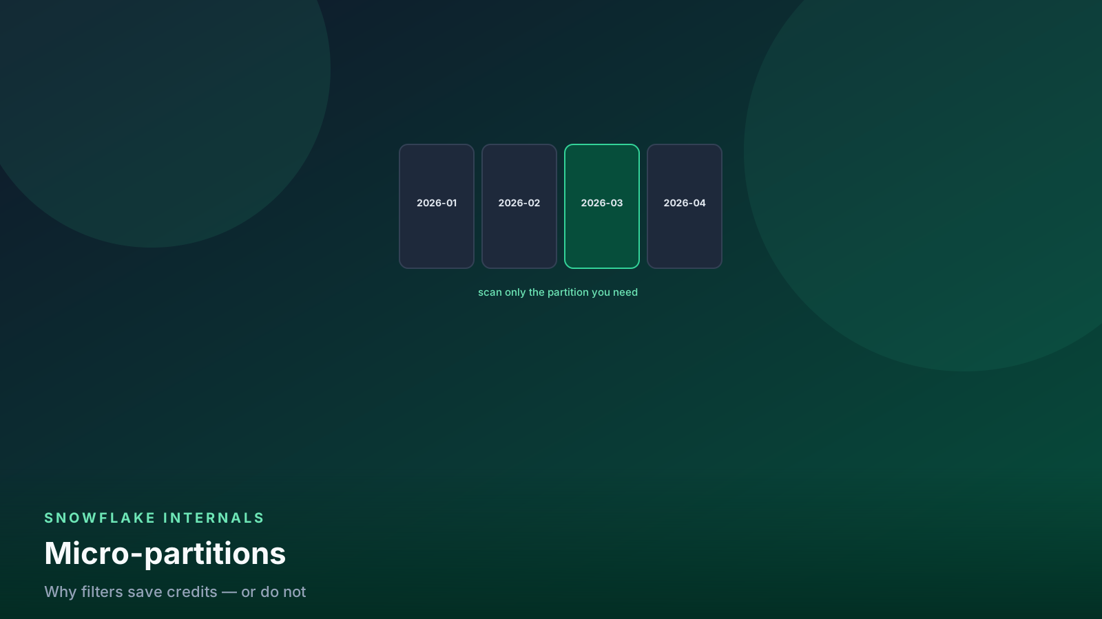
- ✓A micropartition is an immutable columnar file with min/max metadata per column.
- ✓Pruning is metadata comparison. A function on the filter column disables it.
- ✓Clustering is maintenance spend. Use it on large tables filtered the same way.
- ✓SELECT * reads every column in every partition you failed to skip.
- ✓partitions_scanned ≈ partitions_total in query_history is the full-scan alarm.
Table of contents
Snowflake does not store a table as one file. It stores micro-partitions: immutable columnar chunks, typically tens to hundreds of megabytes uncompressed, with min/max (and related) metadata for each column. A query that can prove a partition cannot contain a matching row skips it. That skip is pruning. That skip is most of the performance story.
I do not start a slow-query review with warehouse size. I start with
partitions_scanned versus partitions_total. If those two numbers
are close, the warehouse is scanning a haystack you already had a
magnet for. Size is the last knob — the
cost guide says the same
thing for a reason.
flowchart LR
  q[Query + filter] --> meta[Partition metadata]
  meta --> prune[Skip partitions]
  prune --> scan[Scan the rest]
  scan --> cols[Read named columns]
Metadata first. Bytes second. Warehouse size last.
What a micropartition actually is
Think of a micro-partition as a small columnar file Snowflake wrote
once and will never edit. An INSERT, UPDATE, DELETE, or MERGE
writes new partitions and retires old ones. That is also why
Time Travel works: the old
files stay readable until retention ends.
Each partition carries metadata: the range of values in each column,
approximate distinct counts, and enough information for the optimizer
to decide “this file cannot have event_date = '2026-08-29'.” If the
metadata says the date range is July, the August filter does not open
the file.
You do not pick partition boundaries the way you pick a BigQuery
PARTITION BY column. Snowflake decides the files as you load.
What you do pick is:
- Load order (natural clustering)
- An optional clustering key (maintained clustering)
- Filters that the metadata can compare to
If you came from BigQuery, do not paste a PARTITION BY religion
onto Snowflake. The analog is pruning, not a named partition spec.
BigQuery partitioning
is bytes-scanned billing. Snowflake bills warehouse time. Same
instinct — skip files — different invoice.
Natural clustering is free until it is not
Rows that arrive in date order tend to land in partitions whose date
ranges are tight. A WHERE event_ts >= … AND event_ts < … then
prunes well with no clustering key.
Rows that arrive randomly — a CDC stream keyed by customer_id, a
backfill that wrote three years in one INSERT, a merge that
rewrites half the table — produce partitions whose date ranges span
the whole history. Metadata cannot skip them. Every query becomes a
full scan with extra steps.
I check this before I buy automatic clustering:
select system$clustering_information(
  'analytics.gold.events',
  '(event_date)'
);
The JSON is ugly on purpose. I look at average_overlaps and
average_depth. High overlap means a given date lives in many
partitions. That is the table telling you pruning will fail.
A 20 GB dimension with messy overlap is still not a clustering
candidate. Automatic clustering is a background credit spend. I
cluster multi-terabyte facts that every dashboard filters the same
way — usually a date, sometimes (event_date, account_id).
alter table analytics.gold.events
  cluster by (event_date);

select
  table_name,
  sum(credits_used) as clustering_credits
from snowflake.account_usage.automatic_clustering_history
where start_time > dateadd('day', -30, current_timestamp())
group by 1
order by 2 desc;
If clustering credits exceed the warehouse time you saved, drop the key. Clustering is not a badge. It is a subscription.
Search Optimization is the other paid skip — point lookups, not date-range scans. Do not enable it because a date filter disappointed you. Fix the predicate or the cluster key first.
Wrapping the filter column
Pruning compares the filter to metadata. A function on the column means the optimizer no longer has a range it can compare.
These look innocent. They scan the table:
-- wraps the column: metadata cannot match
select count(*)
from analytics.gold.events
where to_date(event_ts) = '2026-08-29';

select count(*)
from analytics.gold.events
where date_trunc('day', event_ts) = '2026-08-29';

select count(*)
from analytics.gold.events
where year(event_ts) = 2026
  and month(event_ts) = 8;
Write a range on the raw column:
select count(*)
from analytics.gold.events
where event_ts >= '2026-08-29'::timestamp_ntz
  and event_ts <  '2026-08-30'::timestamp_ntz;
Same rows. Metadata can skip. I treat TO_DATE(ts) = … in a hot
query the way I treat a missing WHERE — a bug, not a style choice.
Casting the column to VARCHAR to compare to a string, wrapping it
in LOWER, or joining through a CASE on the fact’s date column
are the same class of mistake. Transform the literal. Leave the
column alone.
-- literal converted, column untouched
select count(*)
from analytics.gold.events
where event_date = to_date('2026-08-29');
If event_date is already a DATE, compare it to a date. Do not
convert the column to text “so it matches the filter.”
SELECT * is a column problem on top of a partition problem
Storage inside a micro-partition is columnar. A query that names
three columns reads three columns from the partitions it did not
skip. SELECT * reads all of them.
On a wide events table — 80 columns, a few VARIANTs — that is
the difference between a dashboard that returns and a warehouse
that runs long. Pruning still matters more: skip partitions first,
then project fewer columns. Do both.
-- production habit on hot paths
select
  event_id,
  account_id,
  event_ts,
  event_name
from analytics.gold.events
where event_ts >= dateadd('day', -1, current_timestamp())
  and event_ts <  current_timestamp();
SELECT * in a worksheet is fine. In a dbt mart that BI reads
every five minutes, name the columns.
VARIANT is its own tax. Snowflake can prune on a scalar column
next to the variant. It cannot skip partitions because you filtered
payload:user_id. Pull the keys you filter on into real columns at
silver. Leave the blob for the columns you rarely read.
flowchart TD
  q[Slow query] --> scan{partitions_scanned ≈ partitions_total?}
  scan -->|yes| wrap{Function on filter column?}
  wrap -->|yes| range[Rewrite as a range]
  wrap -->|no| cluster[Check clustering depth]
  scan -->|no| star{SELECT * or wide VARIANT?}
  star -->|yes| cols[Name columns]
  star -->|no| size[Then consider warehouse size]
Full scan first. Column waste second. Size last.
ACCOUNT_USAGE: partitions_scanned
The number I trust is in query_history. It is lagged. It is still
the Monday habit.
select
  query_id,
  user_name,
  warehouse_name,
  partitions_scanned,
  partitions_total,
  round(partitions_scanned / nullif(partitions_total, 0), 2) as scan_ratio,
  bytes_scanned,
  total_elapsed_time / 1000 as seconds,
  left(query_text, 160) as query_text
from snowflake.account_usage.query_history
where start_time > dateadd('day', -7, current_timestamp())
  and execution_status = 'SUCCESS'
  and partitions_total > 0
order by partitions_scanned desc
limit 30;
scan_ratio near 1.0 on a large partitions_total is the alarm.
A 1.0 ratio on a 12-partition dimension is noise. A 0.98 ratio on
80,000 partitions is the events table.
For “what just ran,” use INFORMATION_SCHEMA query history in the
account. Same columns, shorter lag, shorter retention.
I also look at the Query Profile in the UI: Partitions scanned versus Partitions total. If I am arguing with an analyst about a “slow dashboard,” I screenshot those two numbers before I talk about a Large warehouse.
Bytes scanned next to partition counts tell you whether the leftover partitions are wide. High bytes, low partition ratio: you pruned dates and then read every column. Name the columns.
select
  warehouse_name,
  count(*) as queries,
  avg(partitions_scanned / nullif(partitions_total, 0)) as avg_scan_ratio,
  sum(bytes_scanned) / power(1024, 3) as gb_scanned
from snowflake.account_usage.query_history
where start_time > dateadd('day', -7, current_timestamp())
  and execution_status = 'SUCCESS'
  and partitions_total >= 1000
group by 1
order by gb_scanned desc;
A warehouse with a high average scan ratio is not “the BI warehouse.” It is a SQL problem that happens to live there.
Load shape is a pruning decision
COPY of daily files keyed by date usually produces date-local
partitions. A single INSERT … SELECT that rebuilds three years
produces partitions that each contain a little of everything.
Incremental dbt models that MERGE on updated_at rewrite
partitions that also hold unchanged history. That is normal. It is
also why a clustering key on event_date earns its keep on large
facts: automatic clustering rewrites files in the background so
the next dashboard can prune.
Do not fight this with a nightly full INSERT OVERWRITE. You pay
to rebuild, you pay Time Travel for the old files, and you still
need a cluster key if the overwrite is not date-ordered.
When I backfill, I insert by day (or by week) so each load writes tight partitions:
insert into analytics.gold.events (
  event_id, account_id, event_ts, event_date, event_name
)
select
  event_id, account_id, event_ts, event_date, event_name
from analytics.silver.events_fix
where event_date = '2026-08-01';
Tedious. Cheaper than a three-year file salad.
What pruning is not
- Not a substitute for a filter.
SELECT count(*) FROM eventswill scan the table. That is correct behavior. - Not clustering by default. Clustering is extra. Most tables never need it.
- Not BigQuery partitions. You do not
REQUIRE_PARTITION_FILTER. You write sargable predicates and you reviewquery_history. - Not a reason to disable result cache arguments. Cache hits hide a bad scan until the data ticks. Materialize the grain; do not hope.
Cross-engine comparisons belong in Snowflake vs BigQuery when the question is the invoice shape. This post is the Snowflake-only habit: metadata, then columns, then size.
Pitfalls
TO_DATE(timestamp_col) in the WHERE. The classic. Rewrite
as a half-open range.
Clustering a small table. You pay automatic clustering to re-sort something a Small warehouse already finishes.
SELECT * plus a VARIANT. You skipped no columns and you
decompressed a blob. Name four columns.
Joining on TO_CHAR(date_col). The join key is a function.
Pruning and bloom-style skips both suffer. Join dates as dates.
Reading partitions_scanned on a 20-partition table and
declaring victory. The metric matters when partitions_total is
large.
Buying Search Optimization because a date filter scanned everything. Search Optimization is not a date index. Fix the predicate or the cluster key.
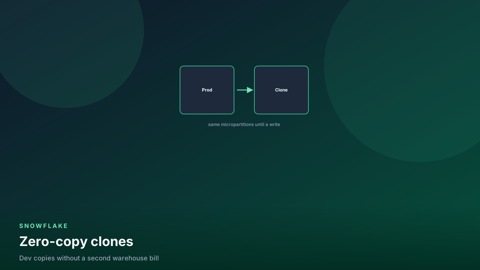
Assuming a clone “inherits” good clustering forever. A zero-copy clone shares files until you write. Heavy DML on the clone creates new, possibly worse, partitions. Check depth after a large merge.
Checklist
When a query is slow or a warehouse spikes:
- Pull
partitions_scanned/partitions_totalfor thatquery_id. - If the ratio is ~1 on a large table, find the filter. Remove functions from the column.
- If the filter is already a range, run
SYSTEM$CLUSTERING_INFORMATIONon the filter column. - Cluster only if the table is large and the filter is stable.
Recheck
automatic_clustering_historyin 30 days. - Name columns on the hot path. Pull filter keys out of
VARIANT. - Only then change warehouse size.
FAQ
Is a micropartition the same as a BigQuery partition?
No. BigQuery partitions are a table property you declare. Snowflake
micro-partitions are files Snowflake writes, with metadata it uses
to skip. You influence them with load order and clustering, not
with PARTITION BY.
Does WHERE date_col IN (long list) prune?
Often, yes, if date_col is bare and the list is actual dates.
A list of TO_DATE(string) literals is still literals. A list
built from TO_DATE(date_col) on the fact side is a wrap.
Will a larger warehouse scan fewer partitions? No. It will scan the same partitions faster (if the job scales). Pruning is a metadata decision. Size is a runtime decision.
How do I see pruning on a worksheet I just ran?
Query Profile: partitions scanned versus total. For history, use
ACCOUNT_USAGE.QUERY_HISTORY (lagged) or INFORMATION_SCHEMA
in the account.
Should every gold fact have a clustering key?
No. Cluster tables that are large, filtered the same way, and
already written with sargable predicates. If
automatic_clustering_history costs more than the queries you
saved, drop the key.
What this means for data engineers
Treat pruning as the first performance review: metadata, then
columns, then clustering, then size. Write ranges on raw columns.
Name the columns a dashboard needs. Read partitions_scanned
every Monday with the rest of the cost worksheet.
A full scan is usually a filter you wrapped or a table you loaded in random order. It is rarely a missing XL warehouse.
Senior Data & AI Engineer · SnowPro Core & Gen AI Certified
4+ years building production data platforms on Snowflake, Databricks, AWS, and Azure. I write from hands-on experience with Medallion architectures, dbt, Airflow, PySpark, and Snowflake Cortex AI. Every tutorial on this blog reflects real pipeline decisions — not documentation rewrites.
Read more about the author →